Find the axis from detected AR
Axis-finding in a planar graph framework
After Detect AR appearances from THR output, a binary mask \(I_k\) representing the spatial region of each candidate AR is obtained. An axis is sought from this region that summarizes the shape and orientation of the AR. A solution in a planar graph framework is proposed here.
A directed planar graph is build using the coordinate pairs
\((\lambda_k, \phi_k)\) as nodes (see Figure Fig. 4 below).
At each node, directed
edges to its eight neighbors are created, so long as the moisture flux
component along the direction of the edge exceeds a user-defined fraction
(\(\epsilon\), see the PARAM_DICT in Input data) to the total
flux. The along-edge flux is defined as:
where \(f_{ij}\) is the flux along the edge \(e_{ij}\) that points from node \(n_i\) to node \(n_j\), and \(\alpha\) is the azimuth angle of \(e_{ij}\).
Therefore an edge can be created if \(f_{ij}/\sqrt{u_i^2+v_i^2} \geq \epsilon\). It is advised to use a relatively small \(\epsilon=0.4\) is used, as the orientation of an AR can deviate considerably from its moisture fluxes, and denser edges in the graph allows the axis to capture the full extent of the AR.
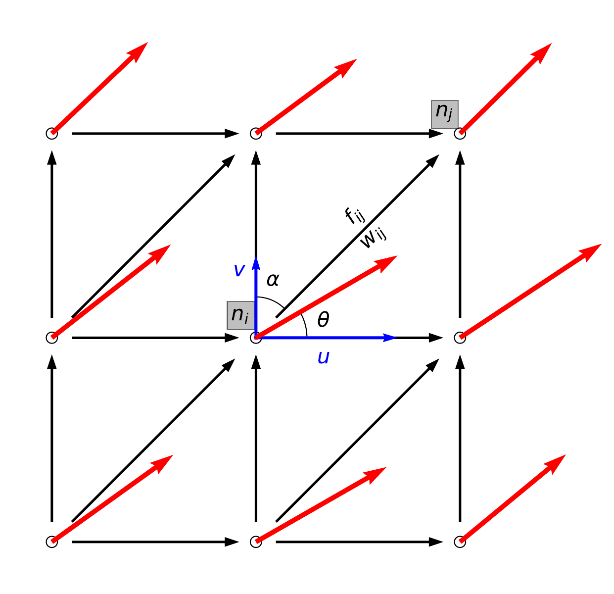
Fig. 4 Schematic diagram illustrating the planar graph build from the AR pixels and horizontal moisture fluxes. Nodes are taken from pixels within region \(I_k\), and are represented as circles. Red vectors denote \(IVT\) vectors. The one at node \(n_i\) forms an angle \(\theta\) with the x-axis, and has components \((u, v)\). Black arrows denote directed edges between nodes, using an 8-connectivity neighborhood scheme. The edge between node \(n_i\) and \(n_j\) is \(e_{ij}\), and forms an azimuth angle \(\alpha\) with the y-axis. \(w_{ij}\) is the weight attribute assigned to edge \(e_{ij}\), and \(f_{ij}\) is along-edge moisture flux.
The boundary pixels of the AR region are then found, labeled \(L_{k}\). The trans-boundary moisture fluxes are compute as the dot product of the gradients of \(I_k\) and \((u_k, v_k)\): \(\nabla I_k \cdot (u_k, v_k)\).
Then the boundary pixels with net input moisture fluxes can be defined as:
Similarly, boundary pixels with net output moisture fluxes is the set
These boundary pixels are colored in green and black, respectively, in Fig. 5.
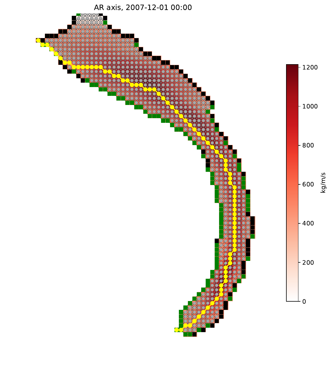
Fig. 5 Application of the axis finding algorithm on the AR in the North Pacific, 2007-Dec-1, 00 UTC. IVT within the AR is shown as colors, in \(kg/(m \cdot s)\). The region of the AR (\(I_k\)) is shown as a collection of gray dots, which constitute nodes of the directed graph. Edges among neighboring nodes are created. A square marker is drawn at each boundary node, and is filled with green if the boundary node has net input moisture fluxes (\(n_i \in L_{k,in}\)), and black if it has net output moisture fluxes (\(n_i \in L_{k,out}\)). The found axis is highlighted in yellow.
For each pair of boundary nodes \(\{(n_i, n_j) \mid n_i \in L_{k, in},\, n_j \in L_{k, out}\}\), a simple path (a path with no repeated nodes) is sought that, among all possible paths that connect the entry node \(n_i\) and the exit node \(n_j\), is the shortest in the sense that its path-integral of weights is the lowest.
The weight for edge \(e_{ij}\) is defined as:
where \(f_{i,j}\) is the projected moisture flux along edge \(e_{i,j}\) and \(A = 100\, kg/(m \cdot s)\) is a scaling factor.
This formulation ensures a non-negative weight for each edge, and penalizes the inclusion of weak edges when a weighted shortest path search is performed.
The Dijkstra path-finding algorithm is used to find this shortest path \(p^*_{ij}\).
Then among all \(p^*_{ij}\) that connect all entry-exit pairs, the one with the largest path-integral of along-edge fluxes is chosen as the AR axis, as highlighted in yellow in Fig. 5.
It could be seen that various aspects of the physical processes of ARs are encoded. The shortest path design gives a natural looking axis that is free from discontinuities and redundant curvatures, and never shoots out of the AR boundary. The weight formulation assigns smaller weights to edges with larger moisture fluxes, “urging: the shortest path to pass through nodes with greater intensity. The found axis is by design directed, which in certain applications can provide the necessary information to orient the AR with respect to its ambiance, such as the horizontal temperature gradient, which relates to the low level jet by the thermal wind relation.
Usage in Python scripts
The following snippet shows the axis finding process:
from ipart.AR_detector import findARAxis
axis_list, axismask=findARAxis(quslab, qvslab, mask_list, costhetas,
    sinthetas, param_dict)
where:
quslab,qvslabare the u- and v- component of integrated vapor fluxes at a given time point.mask_listis a list of binary masks denoting the region of an each found AR.sinthetasandcosthetasare used to compute the azimuthal angles for each grid cell.param_dictis the parameter dictionary as defined in Input data.
Dedicated Python script
No detected Python script is offered for this process, as it is performed in the
AR_detector.findARsGen() function.