Perform the THR computation on IVT data
The Top-hat by Reconstruction (THR) algorithm
The AR detection method is inspired by the image processing technique top-hat by reconstruction (THR), which consists of subtracting from the original image a greyscale reconstruction by dilation image. Some more details of the THR algorithm and its applications can be found in this work of [Vincent1993].
In the context of AR detection, the greyscale image in question is the non-negative IVT distribution, denoted as \(I\).
The greyscale reconstruction by dilation component (hereafter reconstruction) corresponds to the background IVT component, denoted as \(\delta(I)\).
The difference between \(I\) and \(\delta(I)\) gives the transient IVT component, from which AR candidates are searched.
Note
we made a modification based on the THR algorithm as descripted in [Vincent1993]. The marker image used in this package is obtained by a grey scale erosion [1] with a structuring element \(E\), while in a standard THR process as in [Vincent1993], the marker image is obtained by a global substraction \(I - \delta h\), where \(\delta h\) is the pixel intensity subtracted globally from the original input image \(I\).
The introduction of the grey scale erosion process allows us to have a control over on what spatio-temporal scales ARs are to be detected. An important parameter in this erosion process is the size of the structuring element \(E\).
We then extend the processes of erosion and reconstruction to 3D (i.e. time, x- and y- dimensions), measuring “spatio-temporal spikiness”. The structuring element used for 3D erosion is a 3D ellipsoid:
with the axis length along the time dimension being \(t\), and the axes for the x- and y- dimensions sharing the same length \(s\). Both \(t\) and \(s\) are measured in pixels/grids.
Note
the axis length of an ellipsoid is half the size of the ellipsoid in that dimension. For relatively large sized \(E\), the difference in the THR results using an ellipsoid structuring element and a 3D cube with size \((2t+1, 2s+1, 2s+1)\) is fairly small.
Considering the close physical correspondences between ARs and extra-tropical storm systems, the “correct” THR parameter choices of \(t\) and \(s\) should be centered around the spatio-temporal scale of ARs.
Let’s assume the data we are working with is 6-hourly in time, and \(0.75 \times 0.75 ^{\circ}\) in space.
The typical synoptic time scale is about a week, giving \(t = 4 \, days\) (recall that \(t\) is only half the size of the time dimension).
The typical width of ARs is within \(1000 \, km\), therefore \(s = 6 \, grids\) is chosen. Given the \(0.75 \,^{\circ}\) resolution of data, this corresponds to a distance of about \(80 km/grid \times (6 \times 2 + 1) grids = 1040 \, km\). An extra grid is added to ensure an odd numbered grid length, same for the \(t\) parameter: the number of time steps is \(4\, steps/day \times 4 days \times 2 + 1\, step = 33\, steps\).
Compute THR
Using the above setup, the THR process is computed using following code:
from ipart import thr
ivt, ivtrec, ivtano = thr.THR(ivt_input, [16, 6, 6])
where ivt_input is the input IVT data, ivtrec is the reconstruction
component, and ivtano is the anomalous component.
Note
the thr.THR() function accepts an optional argument oro, which is to provide the algorithm with some surface elevation information, with the help of which detection sensitivity of landfalling ARs can be enhanced.
See also
Dedicated Python script
The package provides two script to help doing this computation:
compute_thr_singlefile: when your IVT data are saved in a single file.compute_thr_multifile: when your IVT data are too large to fit in a single file, e.g. data spanning multiple decades and saved into one-file-per year. Like in the case of a simple moving average, discontinuity at the end of one year and the beginning of the next may introduce some errors. When the data are too large to fit into RAM, one possible solution is to read in 2 years at a time, concatenate them then perform the filtering/THR process to achieve a smooth year-to-year transition. Then read in the 3rd year to form another 2-year concatenation with the 2nd year. Then the process rotates on untill all years are processed.
Example output
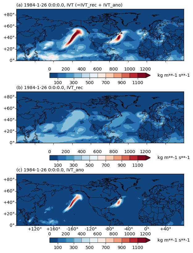
Fig. 2 (a) The IVT field in kg/(m*s) at 1984-01-26 00:00 UTC over the North Hemisphere. (b) the IVT reconstruction field (\(\delta(I)\)) at the same time point. (c) the IVT anomaly field (\(I-\delta(I)\)) from the THR process at the same time point.
References
Footnotes
| [1] | Greyscale erosion (also known as minimum filtering) can be understood by analogy with a moving average. Instead of the average within a neighborhood, erosion replaces the central value with the neighborhood minimum. Similarly, dilation replaces with the maximum. And the neighborhood is defined by the structuring element \(E\). |
| [Vincent1993] | (1, 2, 3)
|